Pattern written by William Thorne · University of Sheffield · National Gallery
Before generative models took over, most machine learning tasks fell into one of two broad categories, and the model you choose depends on the type of task being solved:
Classification - models that sort inputs into categories (e.g. cat vs dog vs bird, or a yes/no decision)
Regression - models that turn inputs into a value on a scale (e.g. a score, or a person’s height)
Ultimately, generative LLMs are just performing classification in a loop. At each step they pick the next token from a fixed vocabulary, which is a classification problem with tens of thousands of categories!
These “classical” methods have not gone away, and for many GLAM tasks they are still the right tool for a number of reasons:
fast - predictions in milliseconds on an ordinary laptop, no GPU required
cheap - no per-call API costs, no expensive hardware requirements
interpretable - you can inspect exactly which words drove a decision
easy to train - models train quickly and reliably on even small amounts of data.
When the task is narrow and you have some labelled examples, a small classical model often beats reaching for a large language model. In this chapter we will use scikit-learn to build a classification model for predicting the artistic style of a painting from its web-text description.
8.1 The Task
The National Gallery Style Classification dataset pairs the National Gallery’s web-text descriptions of paintings with the artistic styles those paintings belong to — Baroque, Gothic, Impressionist, and so on. Our goal is to train a model that reads a description and predicts the style.
Collections are full of free-text descriptions that have never been consistently tagged with controlled vocabulary. A classifier that suggests a style term for each record can quickly annotate large numbers of samples, making them more discoverable to researchers and the public.
Note
This is a text classification task: the input is text, the output is a category. The same recipe works for subject classification, genre detection, language identification, routing enquiries, etc.
8.2 The Dataset
We load the dataset straight from the Hugging Face Hub with the datasets library. It comes already split into train, valid, and test portions — we train on train and report final numbers on test.
from datasets import load_datasetfrom sklearn import set_config# scikit-learn renders a fitted model as a large interactive HTML diagram by# default. That single huge HTML blob trips up document conversion, so switch# to a compact text representation instead.set_config(display="text")ds = load_dataset("wrmthorne/National_Gallery_style_classification")ds
Each row is one painting. The fields we care about are the two text descriptions short_text (a brief summary) and long_text (the full web-text description), and the list of style labels, labels_text. Let’s look at one:
STYLE: ['Early Renaissance']

An elderly man, barefoot and with an impressive grey beard, is perched on a rock, engrossed in a book. This is Saint Jerome, translator of the Bible into Latin. His only companion is an endearing lion which lies peaceably in the corner -- he had tamed it by removing a thorn from its paw.

Bellini painted this subject several times, always using landscape and dramatic lighting to convey meaning. Cliffs tower around Jerome, cutting him off from civilisation (represented by the walled city in the background). A bright light falls on the saint and on the distant towers, but the landscape between them is plunged in shadow.

Recent technical study has confirmed that the painting is by Bellini himself, rather than a follower. Jerome's head is painted with great attention to detail, and if you look closely you can see the individual brushstrokes in his hair and beard.
Notice the labels come as a list. Each painting can belong to more than one style, for instance, a transitional work might be tagged both Gothic and Early Renaissance. We will start simple and come back to multi-label classification a bit later.
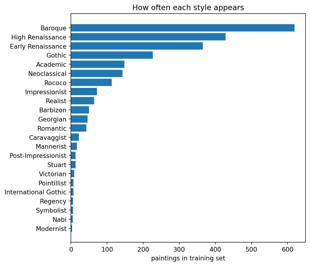
We first want to know what styles are present, and how common is each? The full label set has 23 styles:
from collections import Counterimport matplotlib.pyplot as pltclass_names =sorted({name for row in ds["train"]["labels_text"] for name in row})freq = Counter(name for row in ds["train"]["labels_text"] for name in row)freq =dict(sorted(freq.items(), key=lambda kv: kv[1]))plt.figure(figsize=(7, 6))plt.barh(list(freq), list(freq.values()))plt.xlabel("paintings in training set")plt.title("How often each style appears")plt.tight_layout()plt.show()
This is a heavily imbalanced dataset: Baroque and High Renaissance dominate, while styles like Mannerist, Symbolist, or Victorian appear only a handful of times. This matters a lot for how we measure success, as we will see.
8.3 From Words to Numbers
Models cannot read text directly — it first has to be converted into numbers. This is vectorization. One of the simplest and most effective vectorization methods is TF-IDF (term frequency–inverse document frequency). The idea is simple:
Count how often each word appears in a document (term frequency).
Count the number of documents a word appears in and take its inverse (1/DF = IDF) (inverse document frequency)
Words that appear in lots of documents are not very informative (e.g. “the”, “and”, “or”) and get down-weighted but words that are both frequent in this document and rare across the collection get the highest weight. Here is an example:
from sklearn.feature_extraction.text import TfidfVectorizerexamples = ["A serene Impressionist beach scene at dawn.","A Gothic altarpiece of the Virgin and Child.",]demo = TfidfVectorizer().fit(examples)print("Vocabulary:", list(demo.get_feature_names_out()))demo.transform(examples).toarray().round(2)
Rows are documents, columns are vocabulary words, values are weights. Shared words like “a” wash out while distinctive ones score highly and influence classification more.
8.4 Single Style per Painting
We start with the paintings that have exactly one style, giving us a clean multi-class classification problem to start.
def single_style(split):"""Keep only paintings tagged with exactly one style."""return [r for r in ds[split] iflen(r["labels_text"]) ==1]train_rows = single_style("train")test_rows = single_style("test")len(train_rows), len(test_rows)
(1245, 248)
We chain TF-IDF and a LogisticRegression (confusingly a classifier) into a single Pipeline, so the same steps apply at train and predict time.
from sklearn.pipeline import Pipelinefrom sklearn.linear_model import LogisticRegressiondef xy(rows, field): X = [r[field] for r in rows] y = [r["labels_text"][0] for r in rows]return X, yX_train, y_train = xy(train_rows, "long_text")X_test, y_test = xy(test_rows, "long_text")model = Pipeline([ ("tfidf", TfidfVectorizer(stop_words="english", min_df=2, ngram_range=(1, 2))), ("clf", LogisticRegression(max_iter=1000, class_weight="balanced", random_state=42)),])model.fit(X_train, y_train)
The vectoriser drops English stop words, ignores words appearing in only one document (min_df=2), and keeps bigrams alongside unigrams (ngram_range=(1, 2)) so phrases like “still life” survive. class_weight="balanced" weights the rare styles up, rather than letting the model default to Baroque every time.
NoteRepeatability
Machine-learning code is full of randomness so the same code can give different numbers on different runs. Passing a fixed random_state seeds that randomness, so results are repeatable run-to-run and for anyone else who runs the notebook. Without this, it’s hard to be sure whether an increase in score came from a change you made or just luck.
TRUE:  High Renaissance
PRED:  High Renaissance

The Virgin Mary sits on her mother's lap, her attention focused on the wriggling Christ Child. Her mother, Saint Anne, looks intently at her through deep-set eyes and points upwards to the heavens, indicating the child's divinity. Christ's cousin, Saint John the Baptist, leans against Anne's lap as the baby Christ tickles his chin.

This large drawing was made in preparation for a painting, probab ...
8.5 Did It Work?
One prediction proves nothing. We score the model across the whole test set, against a baseline of always guessing the most common style:
from sklearn.metrics import accuracy_score, f1_scorepred = model.predict(X_test)majority = Counter(y_train).most_common(1)[0][0]baseline =sum(1for y in y_test if y == majority) /len(y_test)print(f"Most-frequent-class baseline : {baseline:.3f} (always guess '{majority}')")print(f"Model accuracy : {accuracy_score(y_test, pred):.3f}")print(f"Model macro F1 : {f1_score(y_test, pred, average='macro', zero_division=0):.3f}")
Most-frequent-class baseline : 0.363  (always guess 'Baroque')
Model accuracy               : 0.823
Model macro F1               : 0.624
While we more than doubled the baseline score, the more important takeaway is the gap between accuracy and macro F1. The difference comes from accuracy rewarding correct classification of common styles where macro F1 averages per style, making it equally important to correctly classify common and rare styles. A high accuracy with a low macro F1 means the model leans on the majority classes and neglects the rare ones. This is why an accuracy figure means little without a baseline to beat.
Let’s inspect the per-class breakdowns:
from sklearn.metrics import classification_reportprint(classification_report(y_test, pred, zero_division=0))
The rare styles, with few or zero training examples, score poorly or not at all. This is a sign to annotate more samples for these labels when using this on your own dataset.
8.6 Short Text or Long Text?
Does the longer text actually help? The pipeline is a few lines, so just train both and compare:
import pandas as pddef evaluate(field): X_tr, y_tr = xy(train_rows, field) X_te, y_te = xy(test_rows, field) m = Pipeline([ ("tfidf", TfidfVectorizer(stop_words="english", min_df=2, ngram_range=(1, 2))), ("clf", LogisticRegression(max_iter=1000, class_weight="balanced", random_state=42)), ]).fit(X_tr, y_tr) p = m.predict(X_te)return accuracy_score(y_te, p), f1_score(y_te, p, average="macro", zero_division=0)pd.DataFrame( {f: evaluate(f) for f in ["short_text", "long_text"]}, index=["accuracy", "macro F1"],).T.round(3)
accuracy
macro F1
short_text
0.754
0.444
long_text
0.823
0.624
Long text wins on both: more words means more information to work with.
8.7 Looking Inside the Model
A linear model assigns a weight to every word, so we can read off which words are most influential for each style:
Note
Some interpretability methods exist for LLMs, but they are typically much more complex, expensive and less informative.
import numpy as npvectoriser = model.named_steps["tfidf"]classifier = model.named_steps["clf"]features = vectoriser.get_feature_names_out()for style in ["Impressionist", "Gothic", "Baroque"]: i =list(classifier.classes_).index(style) top = features[np.argsort(classifier.coef_[i])[-8:][::-1]]print(f"{style:14s}: {', '.join(top)}")
Some of these make perfect sense: Gothic is driven by “virgin”, “christ”, “saint”, “panel”. But notice how many are artist names: Impressionist leans on “monet”, “renoir”, “pissarro”; Baroque on “rembrandt”, “rubens”. The model has partly learned a shortcut by using which artist as a proxy for which style.
That is a real limitation, and the headline accuracy does nothing to inform us of this. Our test set draws from the same pool of artists as the training set, so every time the model leans on “monet” or “rembrandt” it is exploiting a name it has already seen labelled. The test score therefore measures performance on familiar artists, not on style itself. This is only caught by looking inside the model.
To show why this is an issue, we will give the model the Art Institute of Chicago’s description of the impressionist painter Mary Cassatt’s “The Child’s Bath”. Cassatt is not represented in the National Gallery’s permanent collection so she didn’t appear in the training data. Let’s give this to the model to classify:
childs_bath ="""\The Child's Bath is a tender portrayal of familial closeness, a subject thatMary Cassatt explored throughout her career. The caregiver's cheek brushingthe child's shoulder, her encircling embrace, and the child's pudgy hand onher knee suggest an emotional bond between the two.Captivated by a large exhibition of Japanese prints in Paris in 1890, Cassattset out to produce a series of color prints influenced by Japanese aesthetics.She then continued her investigation across media, culminating in this boldcomposition, with its dramatically flattened picture plane, decorativepatterning, and bright palette."""print(f"PRED : {model.predict([childs_bath])[0]}")print(f"'cassatt' seen in train : {'cassatt'in vectoriser.vocabulary_}")
PRED                    : High Renaissance
'cassatt' seen in train : False
The model predicts the wrong style. As seen in the second line, cassatt is not in the vocabulary, preventing the model from exploiting the artist-name shortcut. The model becomes very uncertain without its crutch:
proba = model.predict_proba([childs_bath])[0]for i in np.argsort(proba)[::-1][:5]:print(f"{classifier.classes_[i]:18s}{proba[i]:.3f}")
High Renaissance   0.112
Impressionist      0.104
Early Renaissance  0.096
Baroque            0.096
Neoclassical       0.084
The model is practically random in this instance - no style clears even 12%, despite the text being full of genuine Impressionist signal (“Japanese prints”, “flattened picture plane”, “bright palette”).
8.8 Handling Multiple Labels
Back to the styles we set aside: a painting can hold any number of the 23. The labels field already encodes this as a multi-hot vector — one 0/1 per style, alphabetical, matching class_names. Wrapping LogisticRegression in a OneVsRestClassifier trains one yes/no classifier per style and combines them:
Accuracy is no use here as demanding all 23 labels be exactly right is far too strict. F1 instead trades off how many predicted tags were correct against how many true ones we found. Micro F1 pools every decision (favouring common styles), while macro F1 averages per style (equally weighting the rare classes).
We can now predict several styles for a painting that genuinely has several:
i =next(i for i inrange(len(Y_test)) if Y_test[i].sum() ==2)true = [class_names[j] for j, on inenumerate(Y_test[i]) if on]pred = [class_names[j] for j, on inenumerate(multi_pred[i]) if on]print("TRUE:", true)print("PRED:", pred)
You need predictions to be fast, cheap, and run anywhere
You value interpretability
When to reach for something heavier
The categories are not known in advance, or change constantly.
The signal depends on deep semantic understanding that bag-of-words TF-IDF cannot capture (subtle tone, long-range context, reasoning across the document).
You have very little labelled data but a good description of the task — a zero-shot LLM may do better with no training at all. (The distillation chapter shows how an LLM can be used to generate data to train a small, fast classifier.)
Watch out for
Class imbalance — report macro F1 and a per-class breakdown, not just accuracy, and always compare to a baseline.
Shortcut learning — as we saw, the model may latch onto artist names rather than style. Inspect the top features to catch it.
The ceiling on rare classes — no algorithm rescues a category with three training examples. The answer is more labelled data.